einops

einopseinsum 的使用——einops

​ einops 库操作可以替代全部的张量形状变换操作,注:类似于 Pytorch 中 torch.nntorch.nn.function 的关系,如果像把 rearrange 操作放在 __init__ 中就规定,可以使用 einops.layers.torch 模块中的 Rearrange 函数

einops.rearrange

1
2
ims = numpy.load('./test_images.npy', allow_pickle=False)
# ims中有六张图片,分别为einops的RGB图像

ims 张量的形状为 (6, 96, 96, 3)

1
plt.imshow(ims[0])

png

下面使用einops表示操作过程

矩阵转置:

1
2
3
from einops import rearrange, reduce, repeat
img=rearrange(ims[0], 'h w c -> w h c')
plt.imshow(img)

png

将维度融合操作

1
2
# [6, 96, 96, 3] -> [96, (6 * 96), 3]
rearrange(ims, 'b h w c -> h (b w) c').shape

融合之后的大小为 (96, 576, 3) ,这里 b,w 的顺序很重要,后面进行解释

1
2
# rearrange 不仅仅可以只对一维进行融合操作
rearrange(ims, 'b h w c -> (b h w c)').shape

维度拆分操作

我们将源文件的后三维压缩,视为一张张图片个体,图片在平面中的排列(位置关系)代表着第一维的信息

1
2
3
# 下面操作使将图片的第一维拆分
rearrange(ims, '(b1 b2) h w c -> b1 b2 h w c ', b1=2).shape
(2, 3, 96, 96, 3)

将文件的第一维拆分并融入到 h 和 w 维中

1
2
img = rearrange(ims, '(b1 b2) h w c -> (b1 h) (b2 w) c ', b1=2)
plt.imshow(img)

png

注意这里b1 b2的位置和对应关系很重要,类似于我们的数字表示法,(b1, b2)代表着是在第一维中,每b1个小图片为一个小batch,这些小batch总共会有b2个,那么在上面的例子中,由于顺序是 einops 每三个分组就是 ein 和 ops,再将它们嵌入高宽里面,(b1, h)同样代表着小batch是 h,总共有2个小batch,因此竖着看会有两张图片(把b1嵌入到 h 的维度中去了);同理(b2, w)的情况

1
2
3
# 这种分割方式就是两个图片为一个小batch(哪个b1 b2方向在后面就从哪个嵌入的维度开始排)
img = rearrange(ims, '(b2 b1) h w c -> (b1 h) (b2 w) c ', b1=2)
plt.imshow(img)

png

1
2
3
# 同理将b2 b1在后方交换的情况
img = rearrange(ims, '(b1 b2) h w c -> (b2 h) (b1 w) c ', b1=2)
plt.imshow(img)

png

1
2
3
# 这里在输出中将h放在b1的前面,那么可以看做每张图像的像素每一行互相嵌入 
img = rearrange(ims, '(b1 b2) h w c -> (h b1) (b2 w) c ', b1=2)
plt.imshow(img)

png

1
2
3
# 一个稍微特殊的情况,将图片的宽嵌入到了高里面,相当于把图像拉伸
img =rearrange(ims, 'b h (w w2) c -> (h w2) (b w) c', w2=2)
plt.imshow(img)

png

1
2
3
# w2位于w前,一列共有两个图像(把一个图像密切再重排,这里两个图片只是看起来像,它们拼起来才是原图片)
img =rearrange(ims, 'b h (w w2) c -> (w2 h) (b w) c', w2=2)
plt.imshow(img)

png

einops.reduce

1
2
3
# 在原np操作中,若要对最后一位进行求平均操作要使用x.mean(-1)
# 可以代替为
reduce(x, 'b h w c -> b h w', 'mean')
1
2
3
4
# average over batch
img = reduce(ims, 'b h w c -> h w c', 'mean')
# ims.mean(axis=0)
plt.imshow(img)

png

1
2
3
# 还同时对两个维度进行降维:
img = reduce(ims, 'b h w c -> h w', 'min')
plt.imshow(img)

png

1
2
3
# 甚至可以通过reduce函数进行平均值池化(可以看出reduce里面内置了rearrange函数)
img = reduce(ims, 'b (h h2) (w w2) c -> h (b w) c', 'mean', h2=2, w2=2)
plt.imshow(img)

png

1
2
3
# 压缩通道的例子
img = reduce(ims, '(b1 b2) h w c -> (b2 h) (b1 w)', 'mean', b1=2)
plt.imshow(img)

png

添加或者缩减维度

​ 类似于unsqueeze()操作,在目标张量的某一维中添加维度,可以使用1或者()来进行操作,( ) 表示在新的维度上不显式指明大小

1
2
3
x = rearrange(ims, 'b h w c -> b 1 h w 1 c') # functionality of numpy.expand_dims
print(x.shape)
print(rearrange(x, 'b 1 h w 1 c -> b h w c').shape) # functionality of numpy.squeeze
(6, 1, 96, 96, 1, 3)
(6, 96, 96, 3)
1
2
3
4
5
6
7
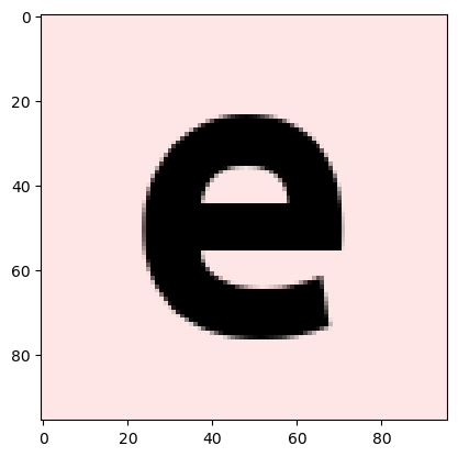
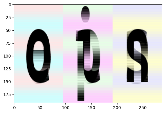
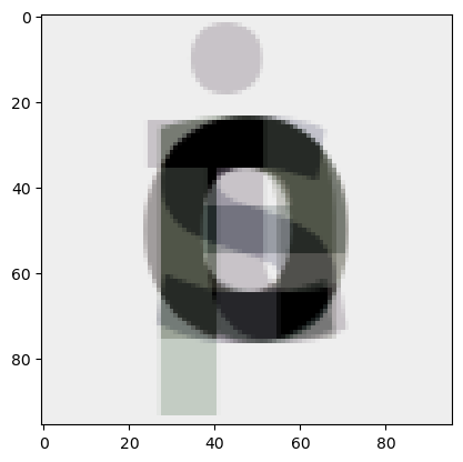
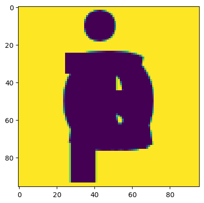
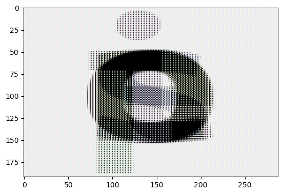
# 先将每张图片最大像素值显现出来,让后转化回去,将其余像素填0 
x = reduce(ims, 'b h w c -> b () () c', 'max') - ims
# 上面的一步没有将维度降下去!!!因为后面与ims进行了计算
# x = reduce(ims, 'b h w c -> b () () c', 'max') 维度变为(6,1,1,3)
# x = x - ims 维度变为(6,96,96,3) 利用了广播操作
img = rearrange(x, 'b h w c -> h (b w) c')
plt.imshow(img)

png

Repeating elements

repeat 用于在某个维度上重复,感觉和 np.repeat 差得不多,没有前面的好用

1
2
3
# repeat along a new axis. New axis can be placed anywhere
repeat(ims[0], 'h w c -> h new_axis w c', new_axis=5).shape
(96, 5, 96, 3)
1
2
# shortcut
repeat(ims[0], 'h w c -> h 5 w c').shape
1
2
3
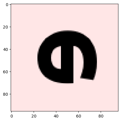
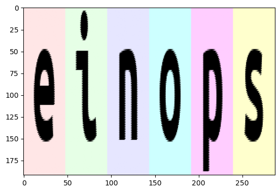
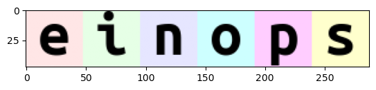
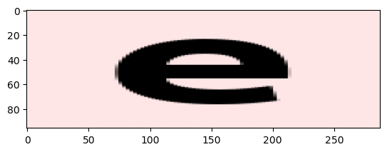
# 同样的repeat中内置了rearrange函数,下面的用法和rearrange一样
img = repeat(ims[0], 'h w c -> h (w repeat) c', repeat=3)
plt.imshow(img)

png

Reduce ⇆ repeat

1
2
3
repeated = repeat(ims, 'b h w c -> b h new_axis w c', new_axis=2)
reduced = reduce(repeated, 'b h new_axis w c -> b h w c', 'min')
assert numpy.array_equal(ims, reduced)
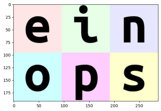
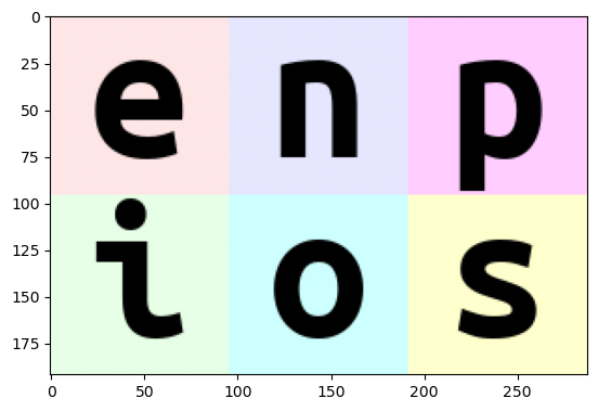
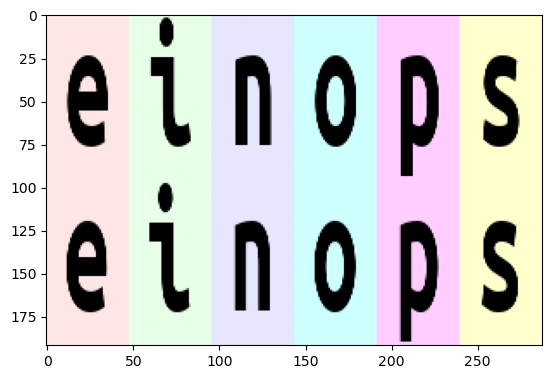
帮助理解的例子

1
2
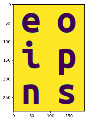
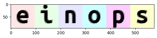
img = rearrange(ims, '(b1 b2) h w c -> (h b1) (w b2) c ', b1=2)
plt.imshow(img)

png

1
2
3
# 一个复杂的例子:
img = rearrange(ims, 'b (h1 h2 h3) (w1 w2 w3) c -> (h1 w2 h3) (b w1 h2 w3) c', h2=2, w2=2, w3=2, h3=2)
plt.imshow(img)

png

Summary

  • rearrange doesn’t change number of elements and covers different numpy functions (like transpose, reshape, stack, concatenate, squeeze and expand_dims)
  • reduce combines same reordering syntax with reductions (mean, min, max, sum, prod, and any others)
  • repeat additionally covers repeating and tiling
  • composition and decomposition of axes are a corner stone, they can and should be used together