dysample

Learning to sample

​ 本文提出了一种新的极轻量级的高效采样算子（比前面所有的都更好，而且是在几乎各个任务中），主要是基于pytorch中grid_sample函数提出。FADE 和 SAPA 对高分辨率图像的需求在一定程度上限制了它们的应用领域，本文避开了动态卷积过程。dysample不需要原始高分辨率的feature map。

提出并优化dysample

​ 设feature map $\mathcal{X} \in \mathbb{R}^{C \times H_1 \times W_1}$，采样集 $\mathcal{S} \in \mathbb{R}^{2 \times H_2 \times W_2}$ ，一维的2表示 $x,y$ 两个坐标，设上采样率为$s$，朴素采样过程为：

$$\mathcal{X'}=grid\_sample(\mathcal{X,S})$$

其中$\mathcal{X'} \in \mathbb{R}^{C \times H_2 \times W_2}$，dysample的想法是引入一个输入和输出分别为 $C$ 和 $2s^2$ 的线性层生成偏移量 $\mathcal{O} \in \mathcal{R}^{2s^2 \times H_2 \times W_2}$，每个采样点由”对应点 + 偏移量“的方式决定上采样图中每个点在采样前图中的坐标，使用F.grid_sample函数，将采样集修改为：

$$\mathcal{S}=\mathcal{O}+\mathcal{G} \\ \mathcal{O}=linear(\mathcal{X})$$

其中 $\mathcal{S}$ 为采样集，$\mathcal{O}$ 为偏移量，$\mathcal{G}$ 为采样对应点，由下面代码生成：

torch.stack(torch.meshgrid([coords_w, coords_h])).transpose(1, 2)

至此就是 dysample 的雏形，下面我们一步步改进 dysample：

修改initial sampling position

​ 由于上采样前后 feature map 大小的差异，上采样后的特征图中有 $s^2$ 个点对应采样前的同一个点，这 $s^2$ 个点的初始坐标都相同，这样就导致了这些点不会区分开来，本质上就是 NN 采样加上了一个偏移量，于是作者将这些点的 initial sampling position 都加上了对应位置的偏离，对于 $s=2$ 的情况，这些点的横纵坐标都分别加上了 $\pm 0.25$，过程如图所示：

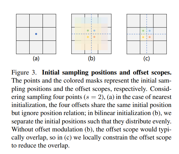
考虑邻域信息：

​ 在dysample中，如果使用 NN 插值上采样，在 $\mathcal{O}=0$ 时那么整个采样过程就等价于NN采样，没有考虑到邻域信息，我们将F.grid_sample 函数中的 mode 调为 bilinear，这样就能考虑邻域信息

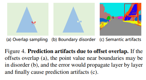
限制偏移量范围：

​ 偏移量过大会导致靠近边界处原有语义簇内的点采样到其它语义簇的情况，这样就会导致边界混乱，因此我们要限制偏移量的范围，使用：

$$\mathcal{O}=0.25linear(\mathcal{X})$$

的方式限定了边界范围，注意：如果使用tanh函数严格控制边界范围反而会导致效果变差，作者在文中给出的解释是太过于严格的边界会限制采样效果，因此在后面中提出了动态边界

减少参数量：

​ 类似于在 nn.Conv2d 中的group操作，我们可以将通道分为 $n$ 个 group，这些 group 内共享参数，作者在文中经验性地说明了$g=4$ 是一种较好的选择

设置动态范围：

​ 将偏移量的范围设置为 $[0,0.5]$ 并以 0.25 为他们的平均值，则偏移量 $\mathcal{O}$ 可继续改写为：

$$\mathcal{O}=0.5sigmoid(linear_1(\mathcal{X})) \times linear_2(\mathcal{X})$$

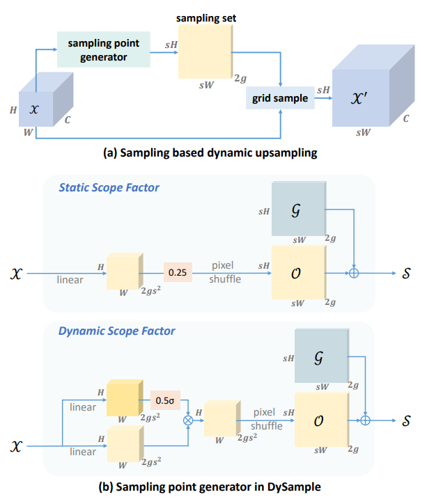
使用PL继续减少参数量

​ 在上面的讨论中，对于每个共享参数的group，我们先使用了CNN生成了大小为 $s^2 \times H \times W$ 大小的偏移量张量，再将其形状变换为 $sH \times sW$ 接得到了符合上采样后大小的偏移量，这个过程称为 “linear + pixelshuffle”（LP），为了减少训练的参数量，我们可以考虑减少通道维数，先进行形状变换操作，即将每个 group $C \times H \times W$ 大小的 feature map 形状变换为 $\frac {C}{s^2} \times sH \times sW$ ，再直接通过CNN生成符合上采样后大小形状的偏移量，这个过程称为 “pixelshuffle + linear” （PL），这样通过减少通道数的方式，我们减少了训练参数量

至此，dysample算子可分为以下四类：

• DySample: LP-style with the static scope factor
• DySample+: LP-style with the dynamic scope factor
• DySample-S: PL-style with the static scope factor
• DySample-S+: PL-style with dynamic scope factor

代码实现：

import torch
import torch.nn as nn
import torch.nn.functional as F
import einops
torch.manual_seed(0)

def normal_init(module, mean=0, std=1, bias=0):
    if hasattr(module, 'weight') and module.weight is not None:
        nn.init.normal_(module.weight, mean, std)
    if hasattr(module, 'bias') and module.bias is not None:
        nn.init.constant_(module.bias, bias)


def constant_init(module, val, bias=0):
    if hasattr(module, 'weight') and module.weight is not None:
        nn.init.constant_(module.weight, val)
    if hasattr(module, 'bias') and module.bias is not None:
        nn.init.constant_(module.bias, bias)


class DySample(nn.Module):
    def __init__(self, c_in, style='lp', ratio=2, groups=4, dySample=True):
        super(DySample, self).__init__()
        self.ratio =ratio
        self.style = style
        self.groups = groups
        self.dySample = dySample
        assert style in ['lp', 'pl']
        assert c_in % groups == 0

        # upsampling 是分为 linear+pixel-shuffle 和 pixel-shuffle+linear
        # downsampling 分为 linear+pixel-unshuffle 和 pixel-unshuffle
        # if ratio > 1:
        if style == 'lp':
            c_out = int(2 * groups * ratio**2)
        else:
            assert c_in >= groups * ratio**2
            c_out = 2 * groups
            c_in = int(c_in // ratio**2)
        
        
        if dySample:
            self.scope = nn.Conv2d(c_in, c_out, kernel_size=1)
            constant_init(self.scope, val=0.)

        self.offset = nn.Conv2d(c_in, c_out, kernel_size=1)
        normal_init(self.offset, std=0.001)


    def Sample(self, x, offset):
        _, _, h, w = offset.size()
        x = einops.rearrange(x, 'b (c grp) h w -> (b grp) c h w', grp=self.groups)
        offset = einops.rearrange(offset, 'b (grp two) h w -> (b grp) h w two',
                                  two=2, grp=self.groups)
        normalizer = torch.tensor([w, h], dtype=x.dtype, device=x.device).view(1, 1, 1, 2)
        
        # offset = torch.zeros_like(offset)

        h = torch.linspace(0.5, h - 0.5, h)
        w = torch.linspace(0.5, w - 0.5, w)
        pos = torch.stack(torch.meshgrid(w, h, indexing='xy')).to(x.device)
        pos = einops.rearrange(pos, 'two h w -> 1 h w two')
        pos = 2 * (pos + offset) / normalizer - 1


        out = F.grid_sample(x, offset + pos, align_corners=False, mode='bilinear', padding_mode="border")
        out = einops.rearrange(out, '(b grp) c h w -> b (c grp) h w', grp=self.groups)
        return out

    def forward_lp(self, x):
        offset = self.offset(x)
        if self.dySample:
            offset = F.sigmoid(self.scope(x)) * 0.5 * offset
        else:
            offset = 0.25 * offset
        if self.ratio > 1:
            offset = F.pixel_shuffle(offset, upscale_factor=self.ratio)
        else:
            offset = F.pixel_unshuffle(offset, downscale_factor=int(1/self.ratio))
        return self.Sample(x, offset)
    
    def forward_pl(self, x):
        if self.ratio > 1:
            y = F.pixel_shuffle(x, upscale_factor=self.ratio)
        else:
            y = F.pixel_unshuffle(x, downscale_factor=int(1/self.ratio))
        offset = self.offset(y)
        if self.dySample:
            offset = F.sigmoid(self.scope(y)) * 0.5 * offset
        else:
            offset = 0.25 * offset
        return self.Sample(x, offset)

    def forward(self, x):
        if self.ratio < 1:
            _, _, h, w = x.size()
            padh = h % 2
            padw = w % 2
            x = F.pad(x, (0, padw, 0, padh), mode='replicate')
        if self.style == 'lp':
            return self.forward_lp(x)
        return self.forward_pl(x)
    
if __name__ == '__main__':
    x = torch.randn(size=(2, 16, 4, 7))
    dy_samp = DySample(16, style='pl', ratio=0.5)
    x = dy_samp(x)
    print(x.size())

代码经验：

• F.interpolate 对某一个通道为 c 进行的 feature map 进行分组插值时，将通道上组的维度移动到 batch 维度上，插值完成之后再从 batch 维度上移动回来即可
• 对于模型中不变的Tensor，可以使用 register_buffer 将 Tensor 保存到模型中
• 使用函数分开各部分的功能提高代码可读性

参考文献：

Learning to Upsample by Learning to Sample